Code & Curiosity: A Developer's Notebook

Crack The Code of Predictions

Ever wondered how companies predict sales based on ad spending? If a company spends $175 on TV ads, how much can they expect in sales? Linear regression helps answer questions like these by identifying relationships between variables. It is one of the simplest yet most powerful tools in data science, commonly used in business, economics, and various analytical fields.

Step 1: Setting Up Your Environment

Before we begin, ensure you have the required Python libraries installed. If you haven’t already, run:

pip install scikit-learn pandas numpy matplotlib

Now, import the necessary libraries:

import numpy as np
import pandas as pd
import matplotlib.pyplot as plt
from sklearn.model_selection import train_test_split
from sklearn.linear_model import LinearRegression
from sklearn.metrics import r2_score

Step 2: Loading and Exploring Data

For this tutorial, we’ll create a simple dataset representing TV ad spending and the corresponding sales generated.

data = {
    "TV_Ad_Spend": [230, 44, 17, 151, 180, 8, 57, 120, 199, 60],
    "Sales": [22, 10, 8, 18, 20, 5, 9, 15, 21, 11]
}
df = pd.DataFrame(data)

Quick Data Check

print(df.head())  # Displays the first five rows
print(df.describe())  # Summary statistics

Step 3: Preparing the Data

We define our independent variable (TV_Ad_Spend) and dependent variable (Sales), then split the data into training and testing sets.

X = df[["TV_Ad_Spend"]]  # Predictor variable
Y = df["Sales"]  # Target variable

# Split into training (80%) and testing (20%) datasets
X_train, X_test, y_train, y_test = train_test_split(X, Y, test_size=0.2, random_state=42)

Step 4: Training the Linear Regression Model

Now, let’s create and train a Linear Regression model.

model = LinearRegression()
model.fit(X_train, y_train)

Understanding the Model Coefficients

print(f"Slope (Coefficient): {model.coef_[0]:.2f}")
print(f"Intercept: {model.intercept_:.2f}")

• Slope (Coefficient): Represents how much sales increase per additional dollar spent on TV ads.

• Intercept: The expected sales when no money is spent on ads.

Step 5: Making Predictions

We now use our trained model to make predictions on the test set.

y_pred = model.predict(X_test)

Step 6: Evaluating Model Performance

To measure how well our model fits the data, we use the R² score:

r2 = r2_score(y_test, y_pred)
print(f"R² Score: {r2:.2f}")

• R² Score: Ranges from 0 to 1, with higher values indicating a better model fit.

Step 7: Visualizing the Regression Line

A visual representation helps us understand how well the model predicts sales.

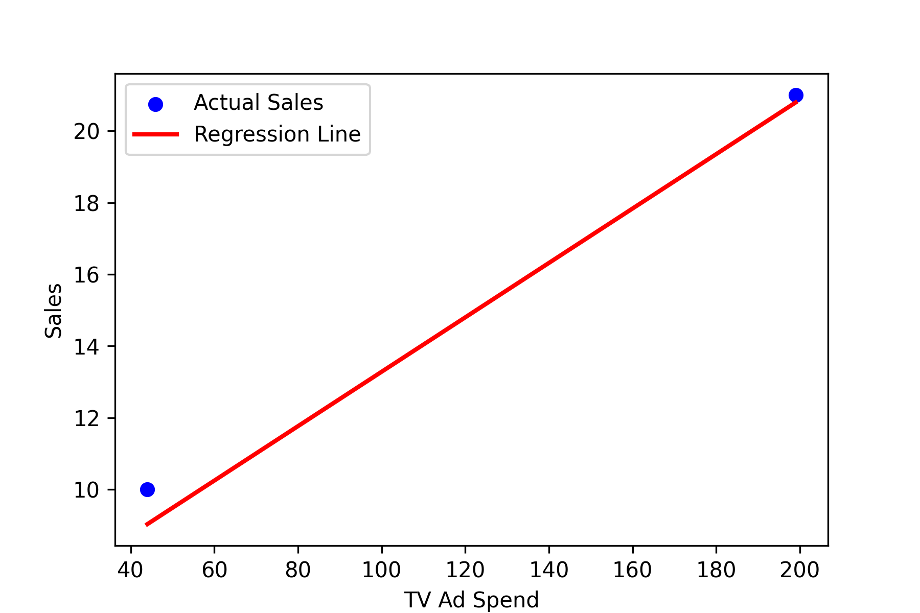
Graph Interpretation

The scatter plot shows actual sales values, while the regression line represents predicted sales. If most points are close to the line, our model makes accurate predictions.

Wrapping Up: What’s Next?

Congratulations! You just built your first linear regression model in Python.

You learned how to:

1. Load and explore data
2. Train a linear regression model using Scikit-Learn
3. Interpret the slope and intercept
4. Evaluate model performance using R²
5. Visualize the results with a regression line

Next Steps:

If you’re looking for a more statistical approach similar to R, consider using statsmodels. It provides additional features like p-values and confidence intervals, which can help assess the significance of your predictors. If these are important for your analysis, statsmodels is a great alternative to Scikit-Learn for regression modeling. Check out Statsmodels’ documentation.